The scourge of scaling

Talk of scale in microbiome studies may take a few different forms. A small-scale study may have a few hundred samples, while a large-scale study is one with tens of thousands.
Or, we might be focusing on physical dimensions, as the scale of a eukaryotic cell tends to be larger (10—100 um), when compared with bacteria (0.5-5 um) and viral particles (100 nm). Similarly, we may be referring to scaling laws, such as the energy theoretic constraints on the size of an organism. We may be talking about scale in very abstract terms, such as how the number of microbes on the planet (1 x 1030) exceeds the number of known stars in the universe (1 x 1024).
One type of scale that lurks behind the scenes, however, and impacts all research design, implementation and interpretation, are computational costs and they manifest their complexity in a variety of ways. Even though data generation is becoming cheaper, these computational hurdles mean that the total cost and time to results is increasing. What is critically needed are investments in software development in order to avoid protracted delays in study timelines.
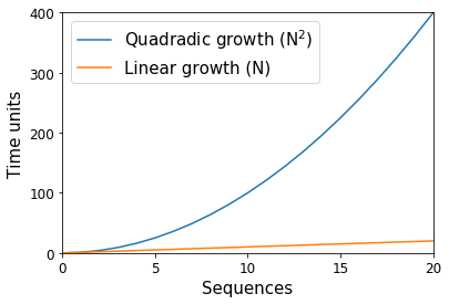
Way back in the dark ages of microbiome science (15—20 years ago), thousands of DNA sequence fragments were considered to indicate a huge study. These sequences were split among tens of samples, with the bulk of time spent on the molecular work necessary to produce the data, and the analytical time spent to ensure that each sequence was accurate and clean of error. At the time, computational algorithms that scaled proportional to the square of the number of sequences (e.g., a quadratic “N2” algorithm) were common — or rather, if we had ten sequences, we would anticipate one of these algorithms to use 100 units, and if we had 20 sequences we would instead anticipate 400 units (Figure 1). With computers, these units are with respect to space (i.e., memory) and time, and they scale separately such that an algorithm may be linear with respect to the number of sequences while exponential in space. In the preceding example, if each unit was 1 kilobyte, ten sequences would need approximately 100 kilobytes of space. Whereas with time, if each unit was 1 minute, ten sequences would need approximately 100 minutes of work.
As you can imagine, these “N2” algorithms presented problems when the number of sequences produced in a study jumped two orders of magnitude with the advent of “next generation” sequencing technologies like the Roche 454 instrument in 2005. In the example above, going from ten sequences to 1000 represents a change from 100 kilobytes of space to 1,000,000 kilobytes (or 100 minutes to 1,000,000 minutes).
That’s nearly 2 years’ worth of minutes, which would have been prohibitive for most labs and bioinformatics teams.
Thankfully, many algorithms can be parallelized in a variety of ways. One of the most frequent forms comes in the decomposition of a problem into small pieces and the orchestration of those tasks over distinct processing elements. This is akin to having a single human read 100 research papers and produce a summary or having ten humans read ten papers each to produce ten summaries that require consolidation. But much like managing humans, the process by which papers are split requires coordination, some humans may be faster than others, and their end outputs need to be rationally aggregated together.
Parallelizing is never simple. So while it probably is the case that using ten humans would produce a result faster, you wouldn’t expect a 10x reduction in the time because of the additional overheads, let alone any serial tasks like having a single person consolidate the summaries so it didn’t read like ten different people wrote it. In computer science, the theoretical improvement with parallelization is known as Amdahl’s law.
Even if our “N2” algorithm above was perfectly parallelizable, so we don’t have to think about all that pesky overhead, and we didn’t care if the produced summary read well, this type of optimization can still be extremely difficult to do well, sometimes requiring specialized software development skillsets. The more complex the program, the more complex this type of optimization is. For the moment, let’s assume we *were* able to parallelize our algorithm perfectly and could distribute over 100 processors. We would then get a result in 10,000 minutes, or about 1 week, which is manageable although frequently in analysis a program is run and rerun many times.
 The Microsetta Initiative in the time of COVID-19
Daniel McDonald and Jack Gilbert discuss the Microsetta Initiative and how it evolved to help in the fight against SARS-CoV-2.
Of course, modern instruments, such as Illumina’s NovaSeq 6000 platform can generate five orders of magnitude more sequence data (6 Tbp) than the Roche 454 GS20 instrument (20 Mbp). If we grow our problem by about the same degree, it would take 19 billion years (and over an exabyte of RAM). Let’s face it, no one is that patient. But, you may think, the program is parallel so it can handle the extra work surely? A computational instrument with 1 billion processors would still take 19 years, and the amount of electricity needed to run a machine like that would be in the gigawatts. Throwing processors at the problem is not the solution.
Herein lies the true complexity: the design and optimization of algorithms and data structure implementations to keep pace with microbiome studies is a massive, often hidden expense. And it is these tools that are fundamental to the essential scientific questions being explored today. This process of taking an existing problem and finding a new way to solve it can take months, years, or potentially be theoretically impossible.
Often, a more scalable approach is more complex, like how a Cessna light aircraft is a much less scalable version than a Boeing 747 jet airplane. Sometimes, revisiting and optimizing the implementation of an algorithm suffices, similar to retrofitting a larger engine into the Cessna. In other circumstances, it may be feasible to balance precision with performance, where an exact solution (e.g., identification of Shiga toxin) may not be required to provide evidence for or against the hypothesis being tested (e.g., whether E. coli O104:H4 is harmful). Nonetheless, much like experimental protocol design, it is a process that takes time, care and a lot of testing.
Thanks to incredible advances in lab automation, miniaturization and high-throughput instruments, the field of microbiome research is now poised to embark on studies that make the Earth Microbiome Project (EMP) look small. Indeed the Original EMP analysis of 28,000 samples is now dwarfed by the >200,000 datasets available publicly through the Qiita database; processing will require over 100x compute relative to the EMP for pairwise operations like sample–sample comparisons. These studies are of immense importance given the variability and shear complexity of the microbiome.
Small sample sizes produce anecdotes. For the study of the microbiome to achieve its potential, it is imperative that studies are able to capture the variance in the modalities of diversity, composition and function that define how microbiomes influence their environment (be that an ocean, soil, plant, animal or human).
If we are to truly understand the diversity of the microscopic, and how those organisms modify the environments in which they reside, we need to substantially increase the scale of our investigations, and also bridge scales so that data on enzymatic processing rates can interact with and influence data on global biogeographic distribution. To this end, we must not forget about the challenge of scaling software to meet these study-driven demands, and instead to meet them head on by budgeting for software developers and experts in optimization when funding microbiome studies in the coming decade.